The following describes a typical workflow for performing an NLLS fit on a single spectrum using the default options. To learn about different options, see the NLLS-Fit Map Options.
-
Select a suitable spectrum display and bring it to the frontmost position in the workspace. Note that if the frontmost data is not suitable, the buttons in the palette will be disabled.
-
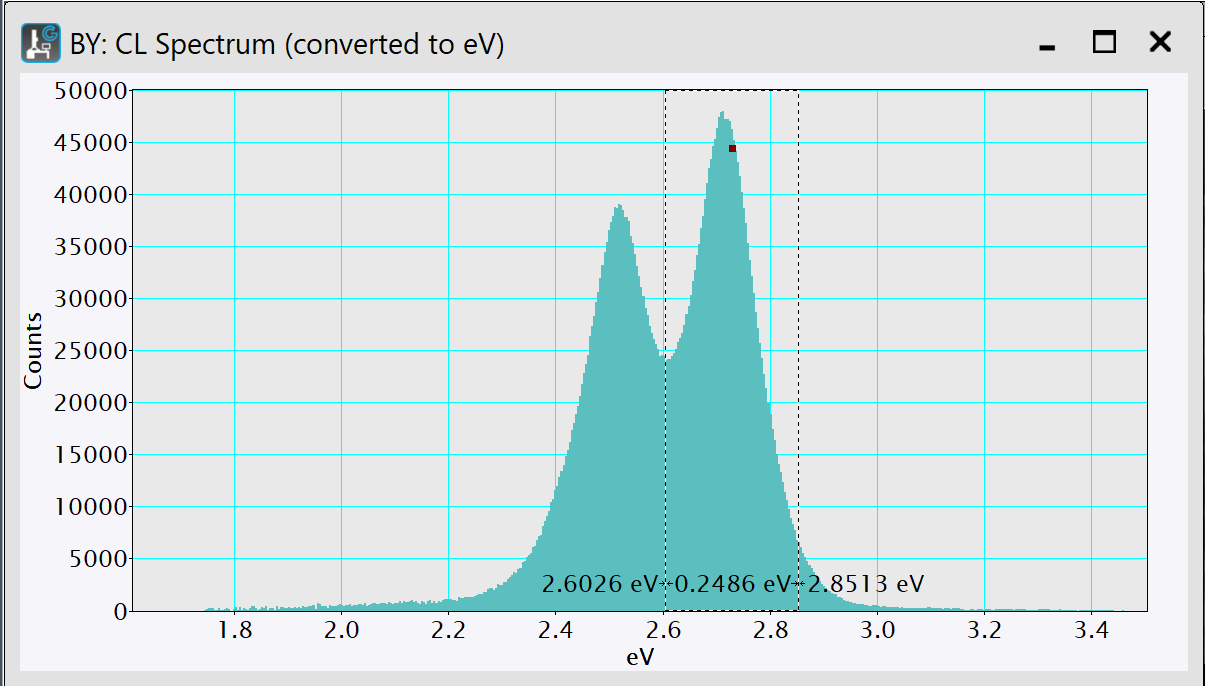
Draw a region of interest (ROI) to designate the area you want to fit.
-
With the data in the frontmost position and the Least-Square Fitting panel in NLLS mode, click the Add model button.
This will add the selected default item to the palette model list. The fit range will be taken from the previously made range ROI. If no such ROI is found, the range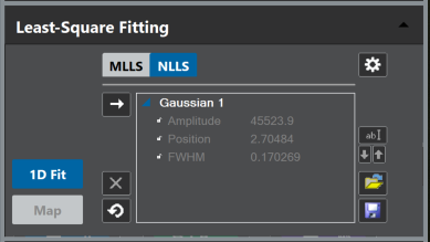 The feature with the highest intensity (for peak models) or the center of the data (for other models) will be automatically chosen.
Note that you can add an item of any type by pressing the Add model button while pressing the ALT key. This will prompt a model-type selection dialog from which to choose. -
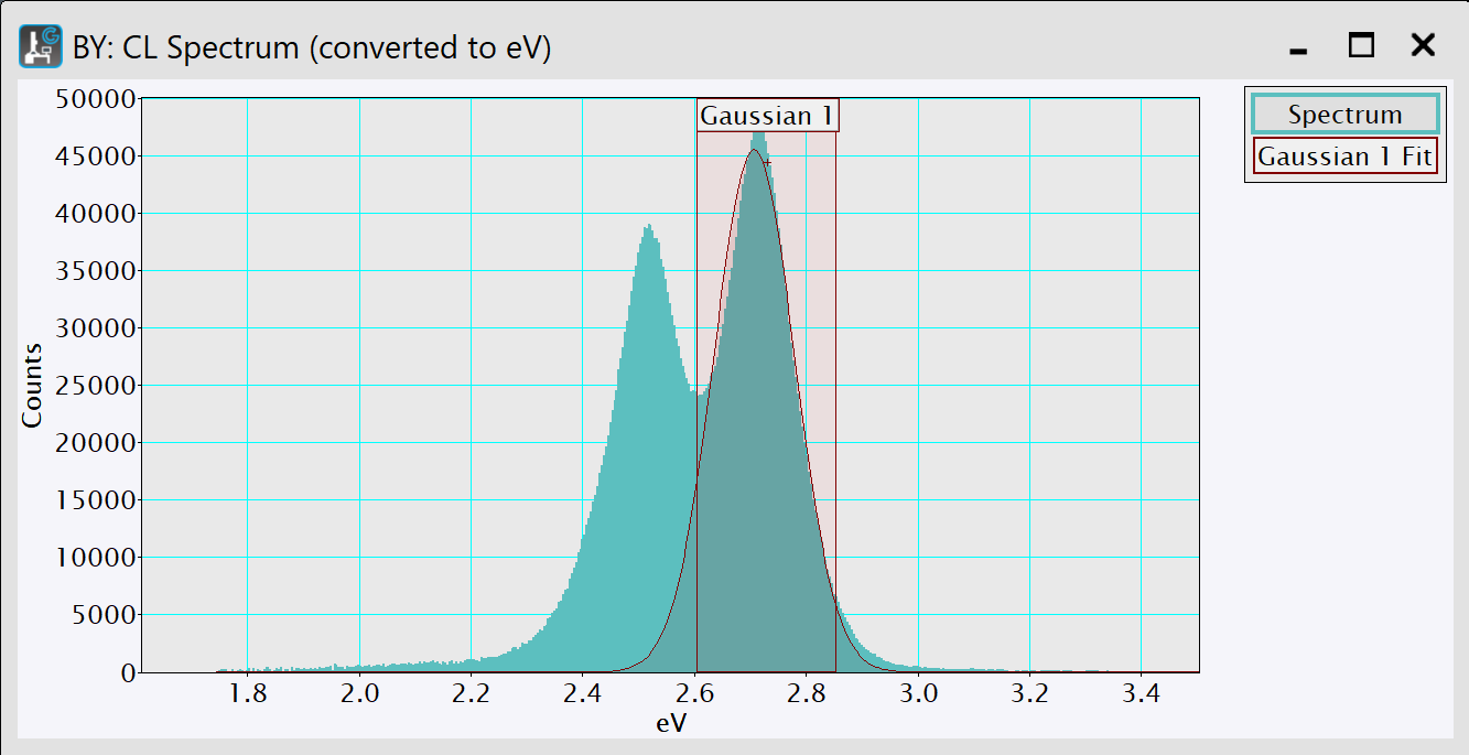
Adding an item to an empty list will automatically enable the live-fit. The data's line plot display will show additional slices presenting the fit results. You can customize the display in the Setup dialog. In addition, you can manually enable or disable the live-fit by pressing the 1D Fit button.
-
Optional: You can adjust the fitting range by resizing the range ROI labeled by the item's name. The fit will automatically recompute.
-
Optional: Resort or rename references in the list. The display will automatically update.
-
Optional: Observe the fit-parameter results by expanding the reference-entries in the model list.
-
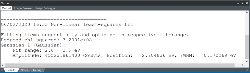
Click the 1D Fit button to output the full fit-results again while pressing the ALT key. The results will appear in the Output window.
-
Optional: Save the model setup for re-applying to different situations using the Save model button.